Recommender System (1) YouTube Recommender
The first post of the Recommender Series.
Introduction
Many of us have been using YouTube frequently. On the homepage, we can always find some videos to watch. I often watch cooking recipes and sports highlights. As a result, YouTube usually presents food or sports channels to me. Sometimes, I can also find some trending videos. So, how did YouTube’s recommender system work? In this post, I will revisit a classic paper that introduces the structure of the YouTube recommender system: Deep Neural Networks for YouTube Recommendations
From the perspective of information retrieval, a recommender system consists of two major components: the candidate generation model and the ranking model. In the example of YouTube, the recommender model is expected to select hundreds of candidate videos from the massive corpus and assign scores to candidates for ranking.

In the paper, the authors list three challenges of building such recommender model for YouTube.
-
Scale: YouTube has a massive user base and video corpus, which demands highly specialized distributed learning algorithms and efficient serving systems.
A recent estimation shows that there are more than 122 million daily active users on YouTube (source). To recommend videos to those users, the inference method must be efficient to meet latency requirements. On the other hand, active users interact with different videos every day and produce new data. We can improve the model with those data. In this case, training the model on a single node might not be feasible due to the data size. Thus, distributed learning algorithms are preferable.
TODO: Will write a post about distributed learning later. -
Freshness: The system should be responsive to recent uploaded content as well as the latest action taken by the users.
There exists a trade-off between new content and well-established content. Without careful design, the recommender could keep presenting vintage videos (e.g. uploaded 8 years ago, 1M+ views, 10K+ thumbs up) to users. Content creators might find it hard to make their recent works stand out. Also, if a user searches for a new topic, the recommender should include relevant videos in the next impression.
-
Noise: In training data, only noisy implicit feedback signals are available. Ground truth of user satisfication is rarely available.
On many occasions, lots of YouTube users do not click the “like” button even if they enjoy the video. The same goes for the “dislike” button. In this sense, relying on explicit feedback will introduce sparse training data. Therefore, developers and managers often need to monitor metrics like click-through rate, video watch time, etc.
System Overview
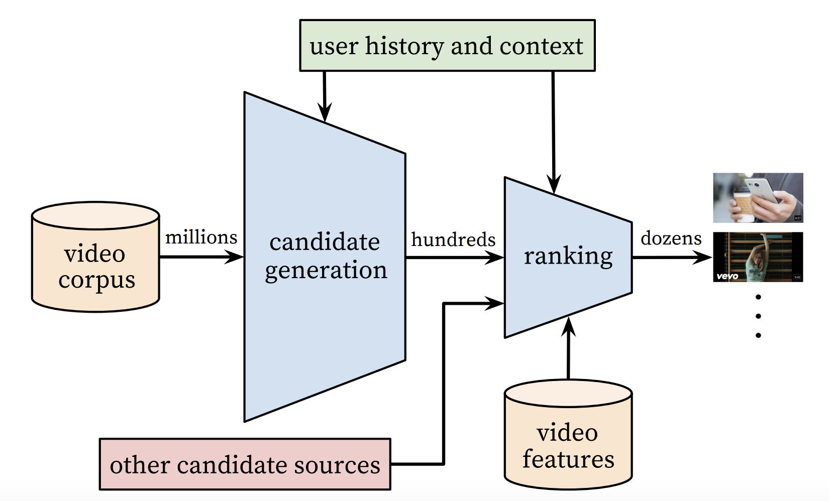
The following figure shows the overall structure of the YouTube recommender system.

As mentioned before, the system consists of the candidate generation network as well as the ranking network. The candidate generation network takes the events from users’ YouTube activity history as input and retrieves a small subset (hundreds) of videos from the large video corpus (millions or more). The ranking network takes in a rich set of features describing the video and user and assigns a score to each video according to an objective function. Highest-scoring videos are presented to the user.
During development, offline metrics (precision, recall, ranking loss, etc.) are used to guide iterative improvements to the system. In production, to determine the effectiveness of an algorithm/model, the authors rely on A/B testing via live experiments. In the experiment, one can monitor click-through rate, watch time, and other metrics that measure user engagement. One interesting observation is that live A/B results are not always correlated with offline experiments.
Design Details
-
Candidate generation network
Take events from the user’s YouTube activity history as input and retrieve a small subset of videos (hundreds) from a large corpus (millions). The objective of this network is to get highly relevant (in the measure of precision) candidates for the user.
This network only provides broad personalization via collaborative filtering. The similarity between users is expressed in terms of coarse features such as IDs of watched videos, search query tokens, and demographics.
-
Ranking network
Its objective is to get a fine-level representation of the candidates and present a few “best” recommendations in a list. The importance of candidates should be assigned with high recall. The ranking network takes in a rich set of features (describing the video and user) and assigns a score to each video according to an objective function. Highest scoring videos are presented to the user.
Candidate Generation
The generation process finds hundreds of videos that may be relevant to users from the enormous corpus. Previously, YouTube was using a matrix factorization approach trained under rank loss
Recommendation as Classification
There are many ways to formulate recommendations. Most of the time, we are predicting whether a positive outcome would happen. For instance, we can define the positive outcome for Youtube recommendation as “User clicks the suggested video”. Then, our objective is to predict the probability of that event.
The authors pose recommendation as an extreme multiclass classification problem. The problem is to accurately predict a specifi video watch $w_t$ at time $t$ among millions of videos $i$ from a corpus $V$ based on a user $U$ and context $C$,
\[P(w_t = i | U, C) = \frac{e^{v_iu}}{\sum_{j \in V} e^{v_ju}}\]where $u \in R^N$ is a high-dimensional embedding of the user, context pair. $v_j \in R^N$ is the embedding of a candidate video. The task of the neural network is to learn user embedding $u$ as a function of the user’s history and context. In this setting, a positive outcome or a positive training example is “a user completing a video”.
There are millions of classes in this problem. If we use all the classes, the softmax layer would be very large and computing the normalization term becomes the bottleneck. The authors relies on a technique to sample negative classes from the background distribution (candidate sampling) and then correct for this sampling via importance weighting
Quick Intro to The Sampling Method Above
The sampling method is originally used under a neural machine translation setting, where there is a large vocabulary set. Prior to training, we partition the training corpus and define a subset \(V^{'}\) of the target vocabulary for each partition. We accumulate unique target words in the training sentences until a predefined threshold $\tau$ is reached.
Then, for partition $i$ with word subset \(V^{'}_{i}\), we can define the following proposal distribution \(Q_{i}\). \(Q_{i}\) assigns equal probability mass to the words in \(V^{'}_{i}\) and zero probability mass to all other words.
Replacing “words” by “videos”, we can derive the sampling method used in the YouTube candidate generation network. For each training example, the cross-entropy loss is minimized for the true label and negative samples within this training partition. In practice, several thousands negatives are sampled.
At serving time, one need to compute the most likely K classes (videos) to present them to the user. The latency requirement could be tens of milliseconds. An approximate scoring scheme sublinear in the number of classes is needed. Previous systems at YouTube relied on Hashing, which is adopted here as well.
Quick Intro to The Hashing Method
- Given a user history and context \(x^{*}\), we use a input partitioner to map it to a set of partitions \(p = g(x^{*})\).
- We retrieve the label sets assigned to each partition \(p_i \in p\). Here, a label is a video. Taking the union of those sets, we have the selected label set: \(L = \cup _{i = 1}^{\|p\|} L_{p_{i}}\), where \(L_{p_{i}}\) is the subset of labels assigned to partition \(p_{i}\).
- At last, we score the labels (videos) \(y \in L\) with the candidate generation network and rank them to produce results.
The input partitioner aims to optimize precision at top \(N\). For more details, please refer to the original paper
In the inference stage, calibrated likelihoods from the softmax layer are not needed. So the problem reduces to a nearest neighbor search problem in the dot product space. To score and rank the candidates, we can use many nearest neighbor search algorithms. The authors claim that A/B test results were not particularly sensitive to the choice of the search algorithm.
Model Architecture
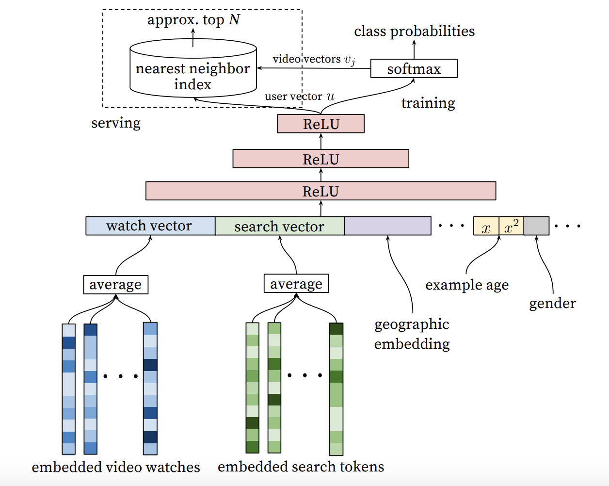
Motivated by the continuous bag of words language models, the authors learn high dimensional embeddings for each video in a fixed vocabulary and feed those embeddings into a feedforward neural network. A user’s watch history is represented by a variable-length sequence of sparse video IDs which is mapped to a dense vector representation via the embeddings. Among the mapping strategies (sum, component-wise max, etc.), taking the average performs the best. The embeddings are learned jointly with all other parameters in the network. Features are concatenated into a wide first layer, followed by several layers of fully connected ReLU.

Input Features
Demographic features are important for providing priors so that we have reasonable recommendations to new users. The geographic region and device features are embedded and concatenated. Simple binary and continuous features (gender, logged-in state, and age) are input directly into the network, normalized into \([0, 1]\).
“Example Age” Feature
In the figure above, you may have noticed that there is a feature named “example age” in the input layer. This feature is introduced to alleviate an underlying issue: a machine learning model tends to exhibit an implicit bias towards the past, as it’s trained from historical examples to predict future results.
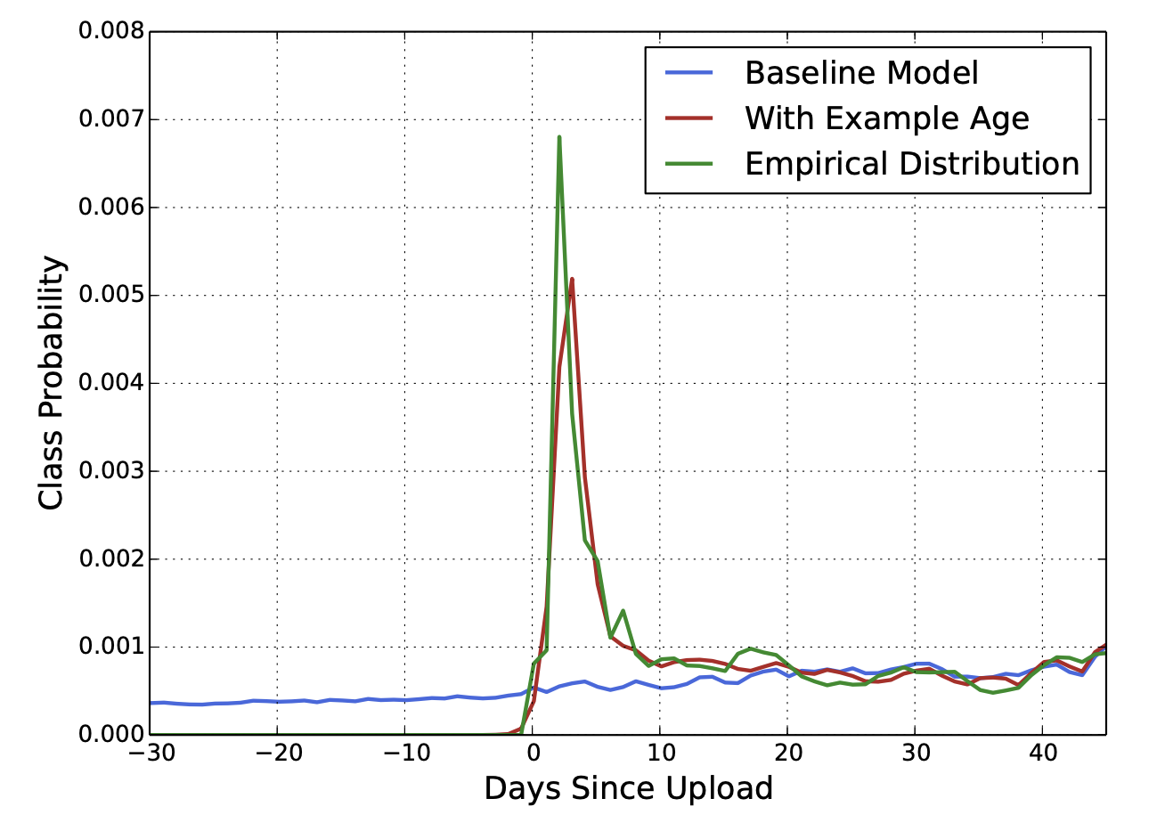
YouTube users prefer fresh content, but not at the expense of relevance. Recommending recently uploaded content to users is important. One challenge is that the distribution of video popularity is highly non-stationary. But the multimodal distribution over the corpus produced by our recommender will reflect the average watch likelihood in the training window of several weeks. In other words, without supplementary signals, the recommender may not recognize the potential popularity of fresh content.
To correct this, the authors feed the age of the training example as a feature during training. At serving time, the age is set to zero (or slightly negative) to reflect that the model is making predictions at the very end of the training window. The figure below shows the effectiveness of this method.

Label and Context Selection
Training examples are generated using all YouTube watches (even those embedded on other sites) rather than just watches on the recommendations the authors produce. Otherwise, it would be hard for new content to surface and the recommender would be overly biased toward exploitation.
Another insight is that generating a fixed number of training examples per user improves live metrics (effectively weighting users equally in the loss function). This prevents highly active users from dominating the loss.
Natural consumption patterns of videos typically lead to very asymmetric co-watch probabilities. Episodic series are usually watched sequentially and users often discover artists in a genre beginning with the most broadly popular before focusing on smaller niches. The authors find much better performance predicting the user’s next match, rather than predicting a randomly held-out watch.
Many collaborative filtering systems implicitly choose the labels and context by holding out a random item and predicting it from other items in the user’s history. This leaks future information and ignores any asymmetric consumption patterns. In contrast, the authors rollback a user’s history by choosing a random watch and only input actions the user took before the held-out label watch. The following figure shows the difference between them.

Ranking
Now, we can use impression data to specialize and calibrate candidates for the particular user interface. For instance, a user may watch a given video with high probability generally but is unlikely to click the homepage impression due to the thumbnail image.
During ranking, we have access to many more features describing the video and the user’s relationship to the video. Ranking is also important for ensembling different candidate sources of which scores are not directly comparable.
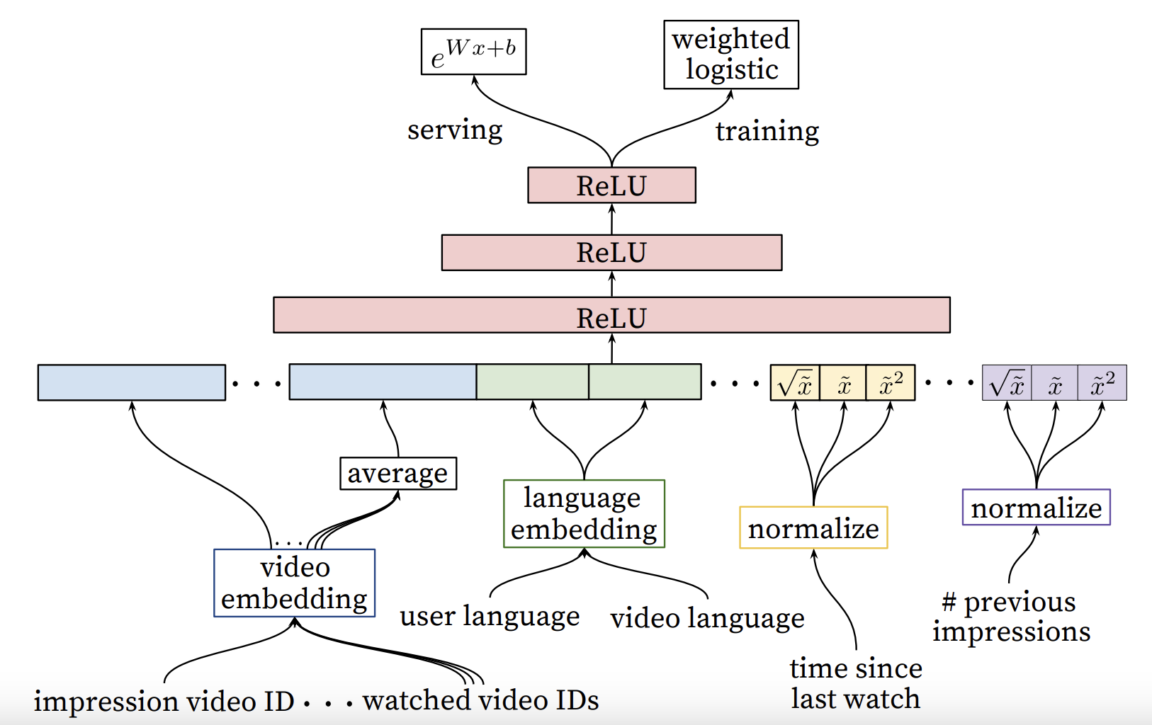
The ranking network architecture is similar to the candidate generation network. It assigns an independent score to each video impression using logistic regression. The list of videos is sorted by the score and returned to the user. The final ranking objective is constantly being tuned based on live A/B testing results. But it’s generally a simple function of expected watch time per impression.
Ranking by click-through rate often promotes click-bait videos. Watch time can better capture user engagement.
The architecture can be represented as below.

Feature Rrepresentation
The features of YouTube have some interesting properties:
- Categorical features may vary widely in their cardinality: some are binary (logged-in status), some has millions of values (users’ last search queries.). Features are further split according to whether they contribute to only a single value (“univalent”) or a set of values (“multivalent”).
Example of a univalent categorical feature is the video ID of the impression being scored, while a corresponding multivalent feature might be a bag of the last 10 video IDs the user has watched.
- Features can also be classified according to whether they describe properties of the item (“impression”) or the properties of the user/context (“query”). Query features are computed once per request while impression features are computed for each item scored.
Feature Engineering
Typically, hundreds of features are used in the ranking model, roughly split evenly between categorical and continuous features. The main challenge is in representing a temporal sequence of user actions and how these actions relate to the video impression being scored. The most important signals are those that describe a user’s previous interaction with the item itself and other similar items.
Consider the user’s past history with the channel that uploaded the video being scored - how many videos has the user watched from the channel? When was the last time the user watched a video in this topic?
These continuous features describing past user actions on related items are particularly powerful because they generalize well across disparate items. The authors also find it crucial to propagate information from candidate generation into ranking in the form of features, e.g. which sources nominated this video candidate? What scores did they assign?
Features describing the frequency of past video impressions are critical for introducing “churn” in recommendations (successive requests do not return identical lists.). If a user was recently recommended a video but did not watch it then the model will naturally demote this impression on the next page load.
Embedding Categorical Features
For categorical features, each unique ID space (“vocabulary”) has a separately learned embedding with a dimension that increases approximately proportional to the logarithm of the number of unique values. Very large cardinality ID spaces are truncated by including only the top \(N\) after sorting based on their frequency in clicked impressions. Out-of-vocabulary values are simply mapped to zero embedding. Multivalent categorical features are averaged before feeding into the network.
Importantly, categorical features in the same ID space also share underlying embeddings. For example, there exists a single global embedding of video IDs that many distinct features use: video ID of the impression, last video watched by the user, video ID that seeded the recommendation. Despite the shared embedding, each feature is fed separately into the network so that the layers above can learn specialized representations per feature.
Normalizing Continuous Features
Proper normalization of continuous features was critical for convergence. Feature values that are equally distributed in (0,1) are desired. The authors used the following method: Assume there is a continuous feature \(x\) with distribution $f$, the normalized feature \(\tilde{x}\) can be expressed as
\[\tilde {x} = \int _{-\infty}^{x} df\]One can approximate the above integral by linear interpolation on the quantiles of feature values.
$x^2, x^{0.5}$ are included for more expressive power, since they can form super- and sub-linear functions of the feature. This could improve offline accuracy.
Modeling Expected Watch Time
The goal of the ranking network is to predict expected watch time given training examples that are either positive (the video impression was clicked) or negative (the impression was not clicked). The model is trained with weighted logistic regression under cross-entropy loss. The positive (clicked) impressions are weighted by the observed watch time on the video. Negative (unclicked) impressions all receive unit weight.
Assuming that we have the probability for a user to click a video as \(p = \frac{k}{N}\), where \(k\) is the number of positive impressions. Now, the odds should look like this:
\[\frac{p}{1 - p} = \frac{k}{N - k}\]With the weighting scheme above, the odds can be further expressed as:
\[\frac{k}{N - k} = \frac{\frac{1}{N}(T_{1} + T_{2} + ... + T_{K})}{1 - \frac{k}{N}} = \frac{E[T_{i}]}{1 - p} \approx E[T_{i}]\]Where \(T_{i}\) is the watch time of the \(i^{th}\) positive impression. Since the click probability \(p\) is usually small on YouTube, the odds is an approximation to the expected watch time. Thus, when serving, we can use the exponential function \(e^{x}\) to produce scores, which closely estimates expected watch time.
In this case, the loss function has the following form:
\[L = - \sum _{i = 1}^{N} (y_{i} w_{i} log(\hat{y}_{i}) + (1 - y_{i}) w_{i} log(1 - \hat{y}_{i}))\]Where \(y_{i} = 1\) if the impression is positive, \(y_{i} = 0\) otherwise.
\(w_{i} = T_{i}\) if the impression is positive, \(w_{i} = 1\) otherwise.
But I haven’t figured out the connection between this loss function and previously deduced odds. If you have some thoughts, please feel free to comment below.